Practical KMeans Clustering with Python
- Introduction
- Generating sample data
- Feature scaling
- Determining $K$
- Model fitting
- Model accuracy
- Conclusion
- Additional links
Introduction
KMeans clustering is perhaps the most well-known technique of partitioning similar data into the same clusters. We take $n$ data points and form $K$ clusters, where $K$ needs to be provided by the user and depends on the dataset. Each cluster has a cluster mean (thus KMeans clustering) and the objective is to minimize each cluster’s variance.
Algorithm
- Choose $K$ number of clusters
- Select $K$ centroids (randomly)
- Assign each data point to closest centroid
- Compute new centroids
- Reassign data points according to new centroids. If no reassignment needed, stop.
With iteration of steps 4) and 5), the centroids will ultimately converge to appropriate centers of the clusters.
Generating sample data
Let’s generate sample data points that can then be used to build clusters. Python’s make_blobs function is helpful in quickly generating the desired points within a 2D space with the desired Gaussian distribution as shown below:
import numpy as np
import matplotlib.pyplot as plt
from sklearn.datasets import make_blobs

centers = [[1, 1], [-1, -1], [1, -1]]
X, y_true = make_blobs(n_samples=500, centers=centers, cluster_std=0.4,
                            random_state=31337)

plt.figure(figsize=(12,9))
plt.annotate('amirootyet.com', xy=(0.03, 0.95), xycoords='axes fraction')
plt.scatter(X[:, 0], X[:, 1], s=50)
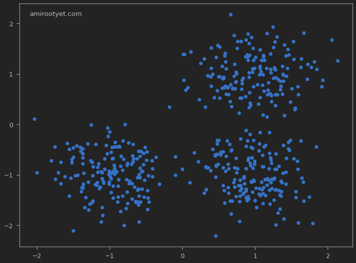
Clearly, we see 3 clusters of data with an isotropic Gaussian distribution. But for the purposes of this exercise, we will assume that we do not know the number of clusters. The next logical step is to determine what the most suitable value for $K$ is in our dataset. But before that, we’ll standardize the dataset.
The array X contains $(x,y)$ coordinates for the generated data points, whereas y_true stores the true cluster numbers. We’ll use y_true later to see how our clustering algorithm performed against this dataset.
Feature scaling
Performing data scaling is essential in order to normalize or standardize data in most datasets. For our dataset, we will use standardization as shown below. There’s no need to standardize y_true since these values will not be used for model training.
from sklearn.preprocessing import StandardScaler

scaler = StandardScaler()
X = scaler.fit_transform(X)
Determining $K$
The visualization clearly shows that there are 3 clusters of data, however a more definitive method of finding $K$ is to run the Elbow method and/or the Silhouette scoring method.
Elbow method
The notion of Within Cluster Sum of Squares (WCSS) is targeted at minimizing the overall distance between points and their respective centroids in the clusters.
$WCSS = \sum distance{(P_i, C_1)}^2 + \sum distance{(P_i, C_2)}^2 + \sum distance{(P_i, C_3)}^2$
Intuitively, we will choose the number of clusters beyond which WCSS or distortions drops are non-significant.
from sklearn.cluster import KMeans

distortions = []
for K in range(1,11):
  clusterer = KMeans(n_clusters=K, init='k-means++')
  model = clusterer.fit(X)
  distortion = model.inertia_
  distortions.append(distortion)

Ks = [i for i in range(1,11)]
plt.plot(Ks, distortions)
plt.xlabel('Number of clusters')
plt.ylabel('Distortions')
plt.annotate('amirootyet.com', xy=(0.75, 0.95), xycoords='axes fraction')
plt.xticks([i for i in range(1,11)])
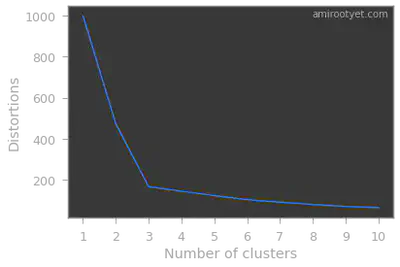
Note that the inertia_ attribute of the KMeans object will provide us the needed distortion or WCSS value.
Silhouette method
from sklearn.metrics import silhouette_score
from sklearn.cluster import KMeans

scores = []
for K in range(2,11):
  clusterer = KMeans(n_clusters=K, init='k-means++')
  model = clusterer.fit_predict(X)
  score = silhouette_score(X, model)
  scores.append(score)

Ks = [i for i in range(2,11)]
plt.plot(Ks, scores)
plt.xlabel('Number of clusters')
plt.ylabel('Silhouette score')
plt.annotate('amirootyet.com', xy=(0.75, 0.95), xycoords='axes fraction')
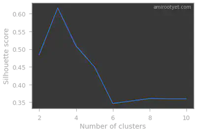
Clearly, in both cases, we see that we have 3 clusters in this dataset. Therefore, during model fitting we will set $K$ to 3.
Model fitting
Now that we know the appropriate number of clusters, $K$, and have standardized our data, we are ready to fit the KMeans clustering model on the dataset. While performing this exercise, keep in mind to use the k-means++ initialization in scikit-learn since it will avoid the trap of poor initial seed values (Random Initialization Trap).
from sklearn.cluster import KMeans

classifier = KMeans(n_clusters=3, init='k-means++', random_state=0, n_jobs=-1)
model = classifier.fit(X)
y_pred = model.labels_
Instead of generating model.labels_ separately, you can also use fit_predict to directly generate the prediction values. Once we have the predicted values, y_pred, we can plot the different clusters to visualize model performance. The converged cluster centers can be accessed using the cluster_centers_ attribute of the KMeans model. This can be helpful if we wish to plot the cluster centroids.
plt.figure(figsize=(12,9))
plt.annotate('amirootyet.com', xy=(0.03, 0.95), xycoords='axes fraction')
plt.scatter(X[:, 0], X[:, 1], c=y_pred, s=50, cmap='Dark2')
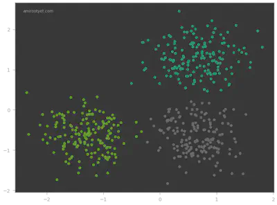
Looks like the KMeans model did pretty well on this dataset! In the next step, we determine exactly how well.
Model accuracy
We compute the accuracy score since y_true holds the true cluster numbers and allows us to compare against ground truth.
from sklearn.metrics import accuracy_score
import numpy as np

print("Accuracy:", accuracy_score(y_true, y_pred))
Accuracy: 0.998
We also build a confusion matrix to visualize where and how many times our model predicted incorrectly.
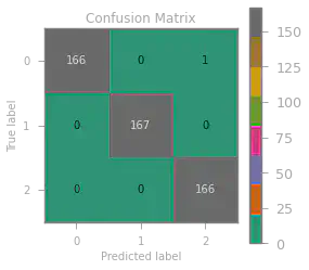
Only one wrong prediction with an accuracy score of $0.998$ – a very accurate model indeed!
Conclusion
Of course, in the real-world, we’ll be unlikely to have a 2D feature set with such a uniform Gaussian distribution. However, this post clarifies the practical application of KMeans clustering with scikit-learn.
Note: The .ipynb pertaining to this exercise is available on my Github here.
Additional links
Pranshu Bajpai
Principal Security Architect
Pranshu Bajpai, PhD, is a principle security architect..